Last year, I introduced the
Accelerated Innovation Community, sponsored by the
MEMS Industry Group, to this space (see “Open-source sensor fusion“). At the time, we were contributing our sensor fusion library to the
MIG GitHub site. Kionix and PNI Sensor Corp. have contributed to the site, and today we
are making another contribution in the form of our trajectory simulation
library.
When my team first started exploring
sensor fusion
topics a few years ago, we needed some way to validate the results of the
algorithms we were looking at. This was before the company had a
gyro, and we didn’t have any kind of motion capture system available to
us. So, we started investigating simulation capabilities. We wanted something
where we could programmatically define a 6DOF trajectory of an object,
including translation in X,Y,Z space, as well as full rotation. Then we needed
sensor models that would take that simulated motion and generate simulated
sensor readings. Those could then be used as inputs of our sensor fusion
simulations. The outputs of those simulations could then be compared with the
original trajectory orientation data to see how well we did.
We found a few tools in the literature, but could not use them for one
reason or another. The
IMUSim tool by A.D. Young, M.J. Ling and D.K. Arvind was of particular interest, but we had trouble replicating the
required software environment. We needed something that could easily be
transferred to other engineers, and decided to write our own
MatlabTM library to do the job. The result was a library of routines
that I collectively refer to as TSim (short for trajectory SIMulator).
The basic idea is to have a good library of functions and canned
routines that can easily be pulled together to succinctly specify motion
in six dimensions. The program listing below shows how I cobbled together the
definition for the motion you see animated at the top of this posting.
  % Copyright (c) 2006-2024, NXP Semiconductors

    path(path, '../tool');
    close all;
    clc;
    outputDir = 'animation_example1_outputs';

    % constant definitions
    sample_rate = 100;               % sensor sample rate
    ts = 1/sample_rate;

    % Define the environment
    env = Env(Env.ENU);

    r = 5*pi();

    % Adata for this test is angular velocity
    %   X     Y      Z
    Adata = [...
        0.0,  r,   0.0;
        0.0,  r,   0.0;
        0.0,  0.0, 0.0;
        r  ,  0.0, 0.0;
        r  ,  0.0, 0.0;
        0.0,  0.0, 0.0;
        0.0,  0.0    r;
        0.0,  0.0,   r];
    Atime = [0; 1; 3; 4; 6; 7; 8; 9];

    % Pdata is position data
    % time   X     Y      Z
    Pdata = [...
        0.0,   0.0,  0.0;
        0.0,   0.0,  0.0;
        1.0,   0.0,  0.2;
        1.0,   1.0,  0.4;
        0.0,   1.0,  0.6;
        0.0,   0.0,  0.8;
        1.0,   0.0,  1.0;
        1.0,   1.0,  1.2;
        0.0,   1.0,  1.4;
        0.0,   0.0,  1.6];
    Ptime = 0:9;

    % Compute parameters for a low pass filter
    % Cutoff frequency=1Hz
    % frequency = 200Hz, 200 taps
    % This filter takes several seconds to run, but does a nice job of
    % ensuring that our waveforms look reasonable.
    % Note that it DOES introduce phase delay (which we don't care about)
    [ N, D ] = LPF( 1, 200, 200 );

    t = CompositeTrajectory('Traj1');
    t = t.set_av('linear', Atime, Adata);
    t = t.set_position('spline', Ptime, Pdata );
    t = t.compute(0.01, 0.005, N, D);
    t.plot_all([1;1;1]);

    t.animate(5, 'animation_example1');
The listing includes two tables. One defines data points of position and time.
The other specifies angular velocity versus time. You probably recall from
your college physics 101 that acceleration is the derivative of
velocity which is the derivative of position. Specify any one of the
three, and the other two can (within a constant value) also be determined.
Angular acceleration, velocity and orientation work the same way.
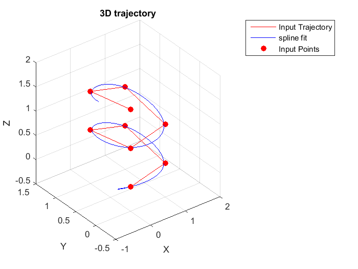
You might think that these tables are pretty crude, but that would be ignoring
the power that Matlab gives us to interpolate between points. We used a
spline function above to create the smooth trajectory shown below.

The basic components of a simulation are:
-
Define the environment: temperature, air pressure, magnetic field, etc.
These can often be left at default values.
- Create a trajectory object to manage the simulation.
-
Define movement and rotation of an object within the environment, link them
to the trajectory object.
- Tell the trajectory object to smooth the trajectory as shown above.
-
Tell the trajectory object to compute sensor outputs based on the simulated
movement and environment.
- Tell the trajectory object to dump outputs.
Because this is a very constrained problem, we’re able to encapsulate
most of the work in the trajectory library itself. That short listing above
was all it took to define the trajectory, dump sensor outputs and create the
animation above.

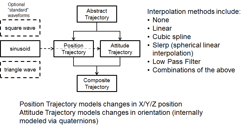
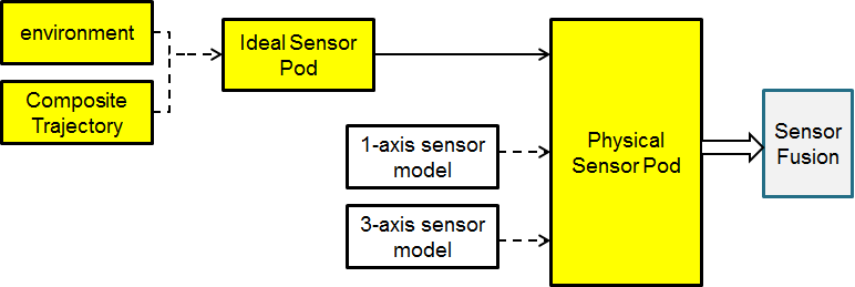
The TSim library makes heavy use of object oriented programming. Trajectory
object construction is shown above. Integration of those
trajectories with sensor models is shown below.

The whole mess is documented in gory detail in the TSim user manual, which is
included in the distribution, which you can download here.
We used TSim as a testbench to characterize our 4.x sensor fusion libraries
last year, and are planning to repeat the process for the recently announced
5.00 fusion libraries in coming months. Our goal is that by making the library
open, we can encourage the sensor fusion community to use a
common collection of stimulus/response datasets for characterization
purposes.
And if you would like to know more about the MIG Accelerated Innovation
Community, please just drop me a line. We’re always looking for new
members.
Michael Stanley “works” on fun sensors and systems
topics.


